Line Intersecting A Polygon

Being able to detect when a line is intersecting a plane will be useful, but I thought next I would have a go at detecting a more specific case: whether or not a line is intersecting a polygon.

For this, I used the same set-up as before: a simple 2D triangle and a line that changes colour based on whether it is intersecting the triangle. Because a line can only be intersecting a polygon if it intersects the plane that the triangle lies on, the code from the program before was reused. First the plane intersection is performed. If the test fails, the line cannot be intersecting the polygon so we are done. If the line is intersecting the plane, we need to perform more analysis to determine if it intersects the polygon.

In order to do this, we first need to determine the point on the plane that the line is intersecting. For this, we need to utilise a vector operation known as the dot product. For arbitrary vectors a and b, the dot product is defined as the following:

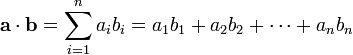
That is, each component of a vector is multiplied together and summed, returning a single value. Given two vectors A and B that represent points in 3D space, the dot product is found by performing the following calculation.

Geometrically speaking, the dot product represents an operation on the length of the vectors and the angle between them. A geometric interpretation of the dot product is as follows:

That is, performing the dot product gives us the lengths of the two vectors multiplied and then multiplied again by the angle between the two vectors. This proves to be a very useful equation for probing the geometric relationship between two vectors. For now, observe that if both vectors a and b are unit vectors, their product will simply be one, meaning that the dot product of two unit vectors will actually give you the cosine of the angle between them.

So how can we use this information to find the point that the line intersects the plane at? Firstly we need a representation of the line to work with so we obtain the line's vector by subtracting one endpoint of the line from the other endpoint. Now that we have the line's vector, we need to find the point at which the vector intersects the plane that the polygon lies on. The first step is to choose one of the line's endpoints and find the   closest distance that it lies from the plane. This is achieved by substituting the endpoint's coordinates into the equation for the plane. We negate the distance value as we want to move back along the vector. This distance is also the magnitude of a vector that shoots perpendicular from the plane to the line's endpoint. Since the normal of the plane is also perpendicular to the plane, the vector from the plane to the endpoint and the plane normal share an orientation. Because of this, we can perform a dot product operation between the normal of the plane and the line's vector to find the angle between the line and the vector from the plane to the line endpoint. After performing these two operations, we now have the angle and the length of one side of the triangle formed between the plane and the line. This is demonstrated below.

Here, we can see that the Line vector L and the Plane Normal N (in the reverse direction because we negated the distance) form a triangle. The use of the plane equation and the dot product have given us the length of one side (-d) and the angle between two of its sides (θ). What we want to find is the magnitude of the side of the triangle from the line endpoint L1 to the intersection point i. This just comes down to basic trigonometry. Since we want to find the length of the hypotenuse and we know the length of the side adjacent to the angle, the length of the hypotenuse can be found by:

This distance tells us how far along the line vector we need to move until we reach the point that intersects with the plane. Geometrically, multiplying a vector by a scalar means moving along the vector. Because of this, in order to obtain the intersection point, we take our endpoint, L1 and add on the line vector multiplied by the magnitude of the distance from L1 to i. This effectively means we start at L1 and move along the vector until we get i.

Now that we have the coordinates of the point where the line intersects with the plane, we have one final step: to determine if that point lies inside of the polygon. To determine the "insidedness" of the point, a simple trick can be performed. Firstly, we visualise drawing lines from each pair of the polygon's vertices to the intersection point. Each pair of lines forms a triangle. This is illustrated in the figure below.

The key to this solution is realising that the angles around the intersection point formed by each of the triangles should all add up to 360 degrees. If the angles do not add up to 360 degrees, the point is not inside the polygon and we can return false otherwise the point is inside the polygon and we can return true. How to construct the triangles within the polygon and find the sum of their angles? The first step is to take two of the vertices and create two vectors originating from the intersection point. This can be done by taking the vertex coordinates and subtracting the coordinates of the intersection point. After normalising, our trusty dot product operation can then be used to find the angle between the two vectors and thus one of the interior angles around the intersection point. Repeating this for each of the polygon vertex pairs and totalling the angles found mean we will be able to determine if the intersection lies inside the polygon or not.

Images: Wikipedia
Images and 3D "insidedness" algorithm: http://paulbourke.net/geometry/insidepoly/

Line Intersecting a Plane

One of the next tasks that I set myself was to write a little demo whereby the intersection of a line with a plane is detected and responded to.

In order to test this, I first used OpenGL to draw a line in space as well as a triangle that could move along the line with the use of the keyboard.

All points on the triangle are coplanar with the plane that is being tested to see whether the line intersects. The goal is to have the colour of the line turn to red once the line is intersecting the plane that the triangle lies on.

After scouring the web, the proved to be a fairly simple process but one that required a few mathematical calculations. The main key to solving the problem is through the use of the equation of a plane:

Where (A,B,C) represents the Normal vector for the plane, (x,y,z) are the coordinates for any point on the plane and D is the distance of the plane from the origin. This equation will evaluate to 0 for any point that lies on the plane. A point not on the plane will yield a result that represents the nearest distance from the point to the plane. If the value is positive, it means the point lies ahead of the plane (in the direction the plane normal points) and if the value is negative, it means the point is behind the plane.

In order to know whether the line is intersecting the plane, we plug the coordinates for the endpoints of the line and plug them into the equation of the plane. By inspecting the distance from the plane of each point, we can determine whether it is intersecting the plane. In order to do this, we need to be able to use the equation for the plane. In order to do that, we need two pieces of information:

• The normal of the plane
• The distance of the plane from the origin (D).

Calculating the Normal of the Plane

The normal of a plane is a vector that is perpendicular to the plane. To make calculations easier, we also normalize the vector, that is making it of length 1. The image below (credit: Wikipedia), shows two normals for a polygon.

In order to calculate the normal for a polygon or plane, we make use of the cross product operation for vectors which takes 2 vectors and returns a vector which is orthogonal to both. This is exactly what we require. Having performed the cross product (and normalizing!), we now have the normal to the plane the coordinates of which are the A, B and C values used in the general equation for a plane. Now we only need D.

Calculating the Distance from the Origin (D)

Once the normal for the plane has been calculated, we need D which is the distance the plane lies from the origin. This is done by simply rearranging the general equation for the plane.

For the (x,y,z) vector, we can use any point on the plane as it would evaluate to 0, allowing us to perform this rearrangement. For the demo, any points used to draw the triangle would suffice.

Checking Line Intersection

We can now calculate a point's distance from a plane using the general equation. How can we use this to check whether a line is intersecting the plane? Well, if the line is intersecting the plane, one of the points will be in front of the plane and one behind. If this is the case, one of the values for the general equation will be positive and the other negative. In order to check whether this is the case, simply substituting the coordinates for each endpoint of the line as the (x,y,z) vector in the general equation and then multiplying the results together. If the line is indeed intersecting the plane, the multiplication will result in a negative number.

Checking for this intersection and drawing the line in the appropriate colour means we are finished!

Camera - Playing with Matrices

So one of the first things I wanted was to have a free roaming camera that would let me explore the world from all angles. I felt this would be very useful for seeing how different things that I had coded would affect the scene and to make sure that there weren't any nasties hiding in a perspective that I hadn't considered!

After playing with OpenGL for a little while, I of course stumbled upon the gluLookAt() function. This takes in 3D world coordinates for the position of the camera and the point that the camera is looking at. The function then constructs vectors from these and does some jiggery-pokery to position the camera at the given coordinates, looking in the direction given, with the world rotated to simulate the camera having moved to that position.

While this was all well and good, I wasn't comfortable with gluLookAt() - it felt too restrictive, too clunky. After looking around the internet, many people commented that for a camera with any real power, managing ones own matrices for world and view transformations was the way to go and in the long run offered more freedom.

I eventually found two very useful websites that helped me learn how to do this:

• The mathematics of the 3D Rotation Matrix - An extensive article by Diane Gruber describing how to construct and maintain 3D rotation matrices to control transformations of the view and world.
• Matrix and Quaternions FAQ - A summary article of various techniques and optimisations when dealing with 3D rotation matrices.

For most purposes, there are two types of camera: a look at camera, and a roaming camera.

Look at Camera

A look at camera is a camera that fixes its view on a single point. This may be a camera that follows the trajectory of a ball as it rotates in a circle.

The first step in building this camera is to construct the 3D rotation matrix. For this purpose, some information is needed: namely, vectors describing the position and orientation of the camera and the world.

To get this information, the user has to provide coordinate information from which vectors can be constructed. These vectors take the following form:

1. Out vector - The vector representing the line of sight of the camera. It is a vector that points from the camera's location to some distant point in the direction the camera is facing. A "look at" vector.
2. Right Vector - This is the vector that is perpendicular to the out vector, originating at the camera's location. It forms the x-axis of the camera's coordinate system
3. Up Vector - This vector is perpendicular to the plane formed by the out and right vectors. It indicates which direction is up relative to the camera.

With these vectors, we know the position of our camera in the world. Together, they can be used to construct the rotation matrix. The rotation matrix is initially constructed by taking the projection of these vectors onto the world coordinate system. The projection onto the world coordinate system merely gives us the end point of each vector, originating from the origin.

The projected coordinates are then used to construct the rotation matrix by having each coordinate of a vector form a row in the rotation matrix (RM). Row 1 in the RM is the right vector, row 2 is the up vector and row 3 is the out vector. 3D rotation matrixes are 4x4 matrices as they make use of homogenous coordinates. This allows translations and rotations to be stored in the same matrix and allows multiplying of matrices whilst preserving any transformations.

The RM is filled in with the negative values for the Out vector as in OpenGL, instead of moving the camera, the world is moved. By default, the camera looks down the negative z-axis, so we minus each of the Out vector coordinates.

So, we use the Out, Right and Up vectors to build the RM but how do we find these vectors?

Finding the out vector is simple. Because we have been given the camera position and look at point by the user, these coordinates define a look at vector with the camera as the origin. To construct the vector, we simply do lookAtPoint - cameraPosition to obtain our Out vector. Simple. We then normalize the vector as dealing with unit vectors simplifies calculations.

Calculating Right and Up are a little more complicated. Once we have our Out vector, we know what the camera is looking at but we have no idea as to what orientation the camera is in - there are an infinite number of rotations around the out vector that could define the camera's orientation.

Knowing the Up vector would fix the orientation but how to find it? The answer lies in defining a reference vector with which to fix the orientation of the camera. This reference vector is called the WorldUp vector and is typically defined as the unit y axis vector of the world coordinates (0, 1, 0).

The WorldUp vector is coplanar with the Out vector. We can then utilise the cross product function to find our Right Vector as the cross product returns a vector that is orthogonal to both input vectors. Since we now have our Out and Right vectors, it is a simple matter of again using the cross product to find the up vector for the rotated camera coordinates. After normalising, we have all the information we need to construct the RM for a look at camera.

One final thing remains to complete our look at camera and that is to perform translation. Translation is performed by creating a translation matrix whereby the amount of translation is contained in the final column of the 4x4 matrix. In the case of the camera, this takes the form of translating the world away from origin (as in OpenGL, the camera stays at the origin and the world is moved). Since we are looking down the x-axis, the world is translated by the negative position of the camera.

>

In order to obtain the final transformation matrix for the world/view, the RM and the translation matrix are multiplied together. Since OpenGL is a right handed coordinate system, the matrices it deals with have their rows and columns swapped. For this reason, the matrix is transposed before being loaded into OpenGL using the glLoadMatrixf(float* matrix) function for use with drawing.

Roaming Camera

The roaming camera utilises Euler angles which specify angles of rotation around the axes. We then construct rotation matrices that produce rotation around each axes. Each rotation is defined as follows.

The final RM that would rotate the world to simulate the movement of the camera is then given by multiplying these matrices together. This process can be optimised however, by noticing that some trigonometric calculations appear multiple times in the final RM. The final RM is evaluated as follows.

Once the RM has been constructed, the translation matrix is constructed in the same way as with the look at camera and the final transformation matrix obtained by multiplying the two and transposing the result.

Relative Rotation

One of the benefits of a roaming camera is to explore the world at will. In order to do this, relative rotation is required - that is, a rotation in respect to the view coordinate system and not the world system. Thankfully this is simple. Once the initial transformation matrix has been constructed, any further rotations applied are relative to the new coordinate system. Relative Motion is thus achieved by multiplying the RM matrix by the new rotation matrix, multiplying the result by the current translation matrix and then loading the final transformation matrix into OpenGL after performing a transpose.

Relative Motion

Moving the camera relative to its coordinate system is slightly more complex. Multiplying a vector by a scalar is the geometric equivalent of moving along the vector by some amount. Using this, relative motion is accomplished by incrementing the amount of translation in the translation matrix by a vector. In order to move the camera forward in the direction it is facing, increase the amount of translation by a scalar multiplied by the Out vector.

Where (x,y,z) is the original amount of translation. The RM is then multiplied by this new translation matrix and the resulting transformation matrix loaded into OpenGL after performing a transpose operation.

(*Images taken from http://www.fastgraph.com/makegames/3drotation/)